This is the final post in a series of interactive-ZK-related research blogs from the Chainlink Labs Research Team. Check out the other posts in the series:

• Introduction to Interactive Zero-Knowledge Proofs
• Background on Computation Complexity Metrics
• Commit-and-Prove ZKs
• VOLE-Based ZK
• VOLE-Based Interactive Commitments
• Realizing VOLE

Author: Chenkai Weng

Contributors: Siam Hussain, Dahlia Malkhi, Alexandru Topliceanu, Xiao Wang, Fan Zhang

Synopsis

In our previous post, we introduced protocols to generate VOLE correlations efficiently using a single-point VOLE (SPVOLE) protocol where the prover’s message is an all-zero vector except at one location. In this post, we describe an efficient SPVOLE protocol.

SPVOLE Functionality

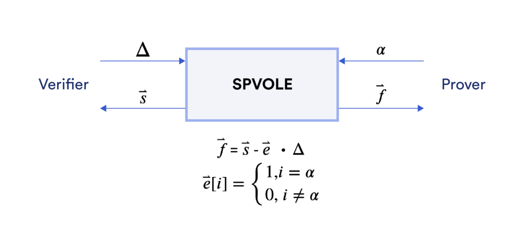
Let’s first recall the functionality of single-point length-$n$ VOLE. It provides a prover with $(\vec{e}, \vec{f})$ and a verifier with $(\vec{s}, \Delta)$, where the Hamming weight of $\vec{e}$ is only 1. They satisfy $\vec{f}=\vec{s}-\Delta\cdot\vec{e}$. It follows that the vectors $\vec{f}$ and $\vec{s}$ contain the same elements at $n-1$ entries, and differ by $\Delta$ at only one entry. 

In detail, it provides a prover with:

• A length-$n$ vector $\vec{f}$ of which all elements belong to $\mathbb{F}_{2^{128}}$.
• A length-$n$ vector $\vec{e}$ of which all elements belong to $\mathbb{F}_2$. The Hamming weight of $\vec{e}$ is only 1 at the entry $\alpha$. This means that $\vec{e}[\alpha]=1$ while all other entries are 0. $\alpha$ is kept secret from the verifier.

Correspondingly, the verifier obtains:

• A global key $\Delta$ that belongs to $\mathbb{F}_{2^{128}}$.
• A length-$n$ vector $\vec{s}$ of which all elements belong to $\mathbb{F}_{2^{128}}$.

These vectors satisfy $\vec{f}=\vec{s}-\Delta\cdot\vec{e}$.

Building Blocks

We will first introduce two building blocks: Oblivious Transfer (OT)¹ and Goldreich Goldwasser Micali (GGM) Construction², before delving into the main construction. Although the protocols mentioned in this post are general two-party protocols, we continue to denote two parties as prover and verifier in order to make it consistent with the previous ZK blog posts.

Oblivious Transfer

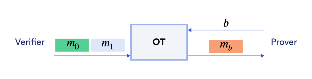
An important building block for SPVOLE is the Oblivious Transfer (OT) protocol. It allows a verifier to select one of two messages provided by a prover without the prover knowing which message has been chosen. As shown in the figure below, the prover inputs two messages $(m_0, m_1) \in \{0,1\}^{2 \kappa}$ and the verifier inputs a choice bit $b \in \{0,1\}$. OT enables the verifier to receive $m_b$ while learning nothing about $m_{1-b}$. It also prevents the prover from learning $b$. In practice, the cost of oblivious transfer is very small thanks to recent advances in OT.

While VOLE can be realized directly by OT with cost linear in the number of correlations, with the help of the Goldreich Goldwasser Micali (GGM) construction discussed below, we can reduce the cost to logarithmic in the number of correlations.

The Goldreich Goldwasser Micali (GGM) Construction

GGM construction was originally designed for converting a length-doubling pseudorandom generator (PRG) $G$ to a pseudo-random function (PRF) $F$. To be more specific, the PRG $G:\{0,1\}^{\kappa} \rightarrow \{0,1\}^{2\kappa}$ takes as input a random seed $k$ of length $\kappa$ bits and outputs $2\kappa$ pseudorandom bits. We denote the first $\kappa$ bits of the output as $G(k)[0]$ and the second $\kappa$ bits as $G(k)[1]$:$$ G(k) \rightarrow G(k)[0] || G(k)[1]$$

A depth-$3$ GGM is demonstrated by the figure below. Starting from the root node, which is the input random seed, the length-doubling PRG $G$ expands each intermediate node into its two child nodes.

1. At level 1, we have
   1. $k_1 = G(k_0)[0]$
   2. $k_2 = G(k_1)[1]$
2. At level 2, we have
   1. $k_3 || k_4 = G(k_1)[0] || G(k_1)[1]$
   2. $k_5 || k_6 = G(k_2)[0] || G(k_2)[1]$
3. At level 3, we have
   1. $F_{k_0}(0) || F_{k_0}(1) = G(k_3)[0] || G(k_3)[1]$
   2. $F_{k_0}(2) || F_{k_0}(3) = G(k_4)[0] || G(k_4)[1]$
   3. $F_{k_0}(4) || F_{k_0}(4) = G(k_5)[0] || G(k_5)[1]$
   4. $F_{k_0}(6) || F_{k_0}(7) = G(k_6)[0] || G(k_6)[1]$

The leaf nodes are the outputs of the PRF $F_{k_0}$. It follows that for any arbitrary $h$-bit input $i$, it only needs $h$ invocations of $G$ to compute $F_{k_0}(i)$.

The GGM construction allows a leaf node to be computed from any node that lies on the path from root to this leaf node. Moreover, a leaf node looks pseudorandom to an adversary who doesn’t know any node on this path.

Constructing SPVOLE From OT and GGM

We will continue using an example to introduce details of the protocol.

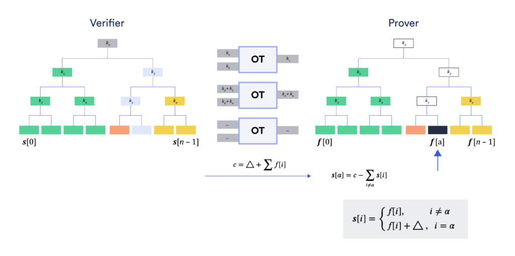
The SPVOLE correlation is generated by leveraging the GGM tree and OT. Assume the verifier (on the left) and the prover (on the right) want to generate an SPVOLE correlation of length 8. The verifier first computes a GGM tree with 8 leaves from a uniform root node. The leaf nodes $(\vec{s}[0],\dots,\vec{s}[7])$ are the output of the verifier. The prover chooses (say) $\alpha = 5$ so she needs to receive $\vec{f}[j] = \vec{s}[j]$ for all $j \neq 5$, and $\vec{f}[5] = \vec{s}[5] – \Delta$. This would make $\vec{f}$ and $\vec{s}$ satisfy the SPVOLE correlation $\vec{f}=\vec{s}-\Delta\cdot\vec{e}$, where $\vec{e} = (0,0,0,0,0,1,0,0)$, i.e., $\alpha=5$.

With a length-8 vector, two parties can use 3 invocations of OT to achieve this. Note that the inverse of bit decomposition of $\alpha$ is $(0,1,0)$, which will be used as the OT choice bits of the prover.

1. During the first OT, the verifier constructs two messages $m_0 = k_1$ and $m_1 = k_2$. The prover inputs the choice bit $\alpha[2] = 0$ and receives $m_0 = k_1$. Then she utilizes the property of GGM tree to expand the whole left sub-tree from its root $k_1$ (marked in green) and gets $(\vec{f}[0],\dots,\vec{f}[3])$.
2. During the second OT, the verifier constructs two messages, $m_0 = k_3 + k_5$ and $m_1 = k_4 + k_6$. The prover inputs the choice bit $\alpha[1] = 1$ and receives $m_1 = k_4 + k_6$. She already knows $k_4$ from the previous step when expanding the sub-tree marked in green, hence she can derive $k_6 = m_1 – k_4$. Then the prover expands the subtree rooted at $k_6$ (marked in yellow) and obtains $(\vec{f}[6],\vec{f}[7])$.
3. During the final OT, the verifier constructs two messages, $m_0 = \vec{s}[0] + \vec{s}[2] + \vec{s}[4] + \vec{s}[6]$ and $m_1 = \vec{s}[1] + \vec{s}[3] + \vec{s}[5] + \vec{s}[7]$. The prover inputs the choice bit $\alpha[0] = 0$ and receives $m_0$. She already knows $(\vec{f}[0],\vec{f}[2],\vec{f}[6])$ from the previous steps when expanding the sub-tree marked in green and yellow, so that she can derive $vec{f}[4] = m_0 – \vec{f}[0] – \vec{f}[2] – \vec{f}[6]$, which is the node marked in pink.

At this point, the prover holds all $\vec{f}[j]$ for $j \neq \alpha$.

Next, the verifier needs to enable the prover to compute $\vec{f}[\alpha] = \vec{s}[\alpha] + \Delta$ without learning $\alpha$. She simply needs to sum up all $8$ elements in vector $\vec{s}$ plus $\Delta$. Specifically, she constructs $c =\Delta + \sum_{j \in [0,7]} \vec{s}[j]$ and sends it to the prover. Upon receiving $c$, the prover subtracts the $n-1$ elements that she already knows to compute $\vec{f}[\alpha] = \vec{f}[5] = c – \sum_{j \neq 5} \vec{f}[j]$.

Security Discussion

For now, we have covered the protocol in the semi-honest setting, assuming that both parties will follow the protocol description. It is not secure against malicious adversaries because, for example, a malicious verifier may not send correct messages to OT, which would lead to the prover reconstructing incorrect values for the GGM-tree. We will discuss how to remove this assumption next, but let’s first appreciate why the above protocol is secure in the semi-honest setting. The security of this SPVOLE protocol stems from the security of GGM and OT. Firstly, GGM ensures that no parent nodes can be deduced from its child nodes. Thus, as long as the prover does not obtain any node lying on the path to $\alpha$-th leaf, it won’t learn the value of $\vec{f}[\alpha]$. This is guaranteed by the security of OT, which ensures that the OT receiver (prover) only learns one message $m_b$ indicated by her choice bit $b$, but not another message $m_{1-b}$. 

Consistency Check

To enhance the protocol to make it secure against malicious players, one needs to perform a consistency check on the validity of the output. Since the output values between the two parties satisfy a linear relationship, we could employ random linear combination to “compress” the number of linear relationships to be checked from $n$ to $O(1)$. This idea is somewhat similar to how one could compress the number of AND-gate checking (via Batch Checking) in the QuickSilver protocol discussed in VOLE-Based ZK.

Conclusion

This concludes our seven-part series on interactive ZK. With this series, we introduced the main advantages of a commit-and-prove ZK, its efficient instantiations based on VOLE, and efficient implementations of VOLE using cheap building blocks. VOLE-based ZKs significantly bring down the cost of zero-knowledge proofs and enable proving multi-billion circuits even on desktop-tier hardware. We see them as an important step in increasing the adoption of ZK technologies in practice, especially when there are already interactions between the prover and the verifier.

¹ Michael O. Rabin, How to Exchange Secrets with Oblivious Transfer, https://eprint.iacr.org/2005/187.pdf

² Oded Goldreich,  Shafi Goldwasser,  Silvio Micali, How to construct random functions, JACM, 1986