Background on Computation Complexity Metrics
This is the second post in a series of ZK-related research blogs from the Chainlink Labs Research Team. Check out the rest of the posts in the series:
Author: Xiao Wang
Contributors: Alex Coventry, Siam Hussain, Dahlia Malkhi, Alexandru Topliceanu, Chenkai Weng, Fan Zhang
In this blog, we will discuss various aspects and metrics of circuits. This will help us understand how to design a scalable ZK protocol. Circuits and Turing machines are two common ways to model a computation. Turing machines are used as mathematical abstractions of our modern computers but are complex to understand; circuits, which contain interconnect gates of basic types, are much simpler. These two models share a lot in common in the set of computations they can describe, though there are some differences. In particular, circuits can only describe bounded computation, while Turing machines can run indefinitely.
Various Computational Complexity Metrics
There are multiple common metrics to measure the complexity of computation. The most common metric is algorithmic complexity, which is the number of steps required to perform the computation. In this post, we will talk about two other metrics.
Representation complexity refers to the amount of information needed to “remember” the computation. When we talk about lines of code or binary size, these metrics are all about the representation complexity of a program. Any computation running in time T can easily be represented in space T by storing each step of the computation. In practice, however, the above worst-case situation rarely happens because most computations have a high degree of uniformity. Uniformity, to put it simply, measures the minimal representation size of a computation. Essentially every program in practice exhibits some level of uniformity. For example, we write functions that can be invoked multiple times. Similarly, a circuit can contain many repeated patterns; in this case, we only need to store one copy of the pattern and dynamically expand the same pattern for different input wires when the circuit is being evaluated.
Runtime space complexity refers to the amount of space (or memory) needed to perform the computation. Runtime space complexity has been studied a lot in computational complexity. For Turing machines, the space needed to execute a program is often sublinear in the execution time. For example, it has been taken for granted that given bounded memory, we can run programs for an essentially unbounded amount of time (of course, assuming there is no memory leak!). However, this is less obvious when the computation is represented as a circuit: Given an arbitrary circuit, at any point, any wire that has been evaluated could be used as the input wire to the next gate. Therefore, without looking ahead, one needs to store information about essentially every wire until the computation is done. As a result, this means that evaluating a circuit, in general, would need memory linear in the circuit size (i.e., linear to the algorithmic complexity). This is one of the root causes of the high memory cost in many cryptographic protocols, which we will expand on soon.
The connection between representation and runtime space complexities. Representation complexity measures the space needed to store the circuit (e.g., lines of code, binary size, etc.); runtime space complexity, on the other hand, refers to the space needed to execute the circuit at runtime. As we discussed above, uniformity in representation complexity is often achieved when the computation has repetitive components. When there is a high level of uniformity, the runtime space complexity tends to be smaller. When uniformity is high, many parts of the computation can be represented as a common subcircuit. Even without uniformity, if a certain part of the computation is done in a function, the space used to compute this function can be overwritten upon completion of the function: Intermediate values in the function will not be needed after the completion of the function. Therefore, if there is a mechanism to deallocate space, repeated calls to the same function only need space needed to evaluate the function once. Alternatively, for circuits, it means that repeated evaluations of the same circuit pattern on different inputs only need space for one evaluation. Crucially, to achieve great runtime space complexity, it is important to allow the deallocation of space.
Examples
A Simple Circuit
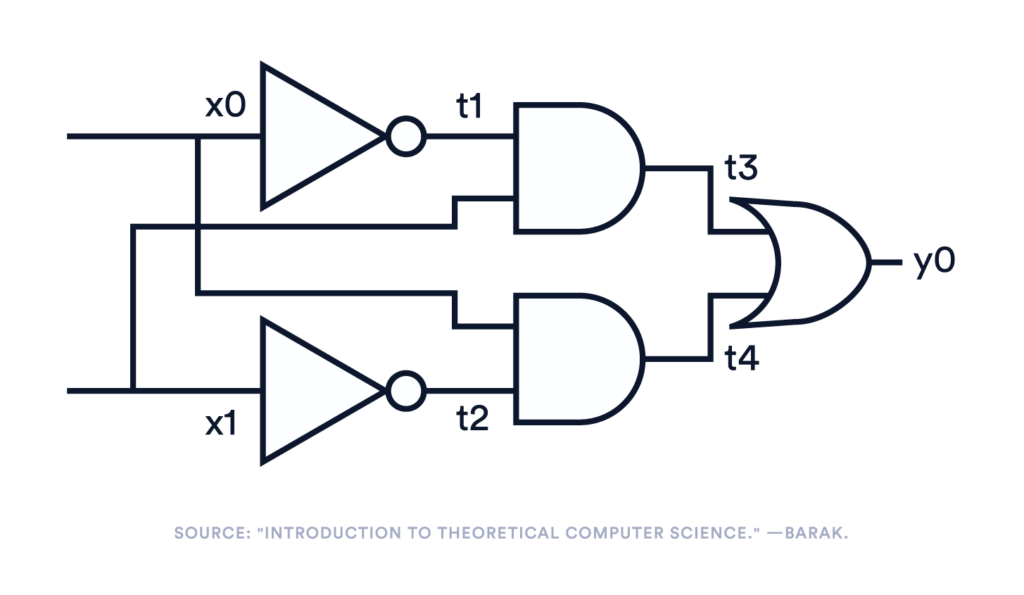
We have been talking a lot about abstract concepts. Let’s use a basic example for illustration. In this example, we will use straight-line programs to represent circuits. A straight-line program, intuitively speaking, is a sequence of steps, each operating on one or more input variables and computing an output variable using a basic gate (e.g., AND/XOR/NOT). For example, in Figure 1, the left-hand side is a circuit with five gates and seven (circuit) wires; the right-hand side is a straight-line program that represents exactly the same computation in five lines.
 |
|
Figure 1. Circuits and straight-line programs.²
A Circuit With Uniformity
Normally, the number of lines in a straight-line program is the same as the circuit size, but when there is some form of uniformity, this can be reduced. As we argued above, this uniformity leads to better runtime space complexity.
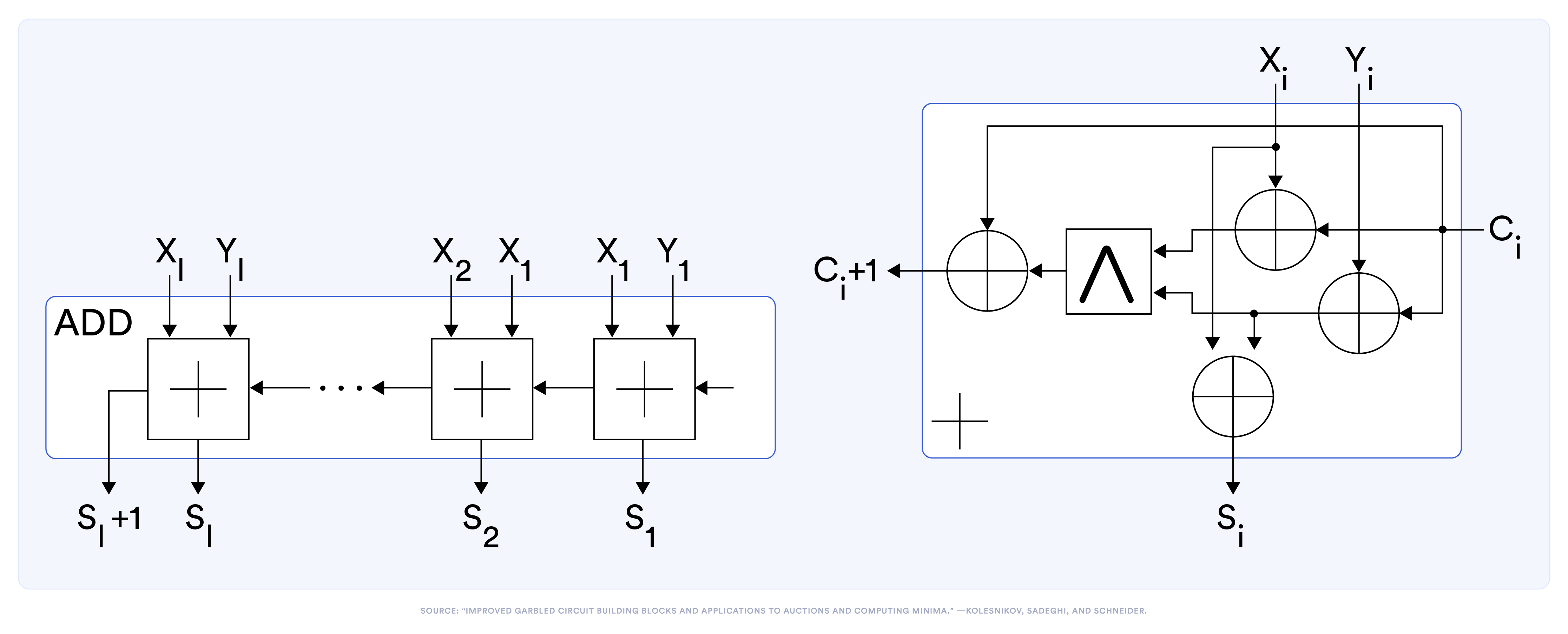
Figure 2. Circuit representation of an ℓ-bit adder and a full adder.³
Take an ℓ-bit adder in Figure 2 as an example. The left side shows the circuit that adds two ℓ-bit numbers. Internally, it contains ℓ copies of the sub-circuit shown on the right side for a full adder that adds two bits. We can write a full-adder in a straight-line program as:
| % co, s <- fullAdder(xi, yi, ci): |
| t1 = XOR(xi, ci) |
| t2 = XOR(yi, ci) |
| t3 = AND(t1, t2) |
| c{i+1} = XOR(t3, ci) |
| si = XOR(xi, t2) |
One can write an ℓ-bit adder in 5ℓ steps in a similar way. When ℓ=3, it would look like the following:
| % s{1…4} <- 3-bit–adder(x{1…3}, y{1…3},c1) : | |
| t1 = XOR(x1, c1) | |
| t2 = XOR(y1, c1) | |
| t3 = AND(t1, t2) | |
| c2 = XOR(t3, c1) | |
| s1 = XOR(x1, t2) | |
| t4 = XOR(x2, c2) | |
| t5 = XOR(y2, c2) | |
| t6 = AND(t4, t5) | |
| c3 = XOR(t6, c2) | |
| s2 = XOR(x2, t3) | |
| t7 = XOR(x3, c3)< | |
| t8 = XOR(y3, c3) | |
| >t9 = AND(t7, t8) | |
| c4 = XOR(t9, c4) | |
| s3 = XOR(x3, t4) | |
It uses nine temporary wires to hold intermediate values.
The above representation contains a great deal of repetition, which intuitively seems redundant. Indeed, one can introduce functions and public-bound loops to “compress” the above representation. In particular, given the function
co, s <- fullAdder(xi, yi, ci), an ℓ-bit adder can be represented as a loop calling this function iteratively.
% ℓ-bitAdder( ..params..):
c = 0
For i in [1, …, ℓ]:
c, si <- fullAdder(xi, yi, c)
s{ℓ+1}=c
We can see that now the program representation is much more succinct than full straight-line programs, but what’s more important is that it also encodes information about the lifespan of many circuit wires. Recall that evaluating a circuit could take memory linear in the circuit size because any wire could be needed at any time; however, when we introduce functions, temporary variables local to the functions do not need to be remembered beyond the scope of that function. On modern computers, it corresponds to the fact that we pop the execution stack when we return from a function. Indeed, although an adder contains 5ℓ gates, the above loop-based representation can be evaluated using just five memory slots in addition to the input/output wires.
Memory Complexity in ZK
We took a detour on computational complexities to understand how uniformity affects the representation complexity and runtime space complexity of a computation. Now we want to apply these facts to figure out what kinds of ZK could enjoy memory friendliness.
First, we remark that one of the drawbacks of most succinct ZK is that memory is linear in the number of gates/constraints in the input statement. This is usually because these protocols need to encode the entire computation in a flattened circuit and then put them in a small number of commitments. It should be noted that some recent work sheds light on possible ways to improve this memory complexity by incrementally compressing the proof at a cost of higher computational overhead or assuming a circuit-emitting oracle. Other solutions include using multiple machines, each of small memory, to jointly prove a large statement that could not fit into one machine.
Luckily, the situation with regards to interactive ZK proofs is much better. From the discussion above, we can see that it is important to be able to “forget” values after they cease to be needed. Intuitively, we want the prover and the verifier to maintain a snapshot of what is proven in the circuit, and this snapshot should be updatable. One way to allow this is via the commit-and-prove paradigm, first discussed by Kilian (89, in his dissertation) and formalized by Canetti, Lindell, Ostrovsky, and Sahai (STOC 02’). We will cover more details regarding this in the next post.
¹When the circuit can be preprocessed, the runtime space complexity to evaluate a circuit is highly related to another concept called “pebbling game.” When the circuit cannot be preprocessed (i.e., the circuit is not known until evaluation), then minimizing runtime space complexity is even more difficult.
²From https://files.boazbarak.org/introtcs/lec_03_computation.pdf
³From “Improved Garbled Circuit Building Blocks and Applications to Auctions and Computing Minima”


